Implementing Sorting Algorithms Pt. II
This post is going to circle back to the topic of sorting algorithms. In a recent post we looked at bubblesort and quicksort of arrays and in this post I’d like to come back to the discussion of various array sorting algorithms. I don’t want to sound like a broken record, but I’ve really been enjoying digging deeper into basic array sorting algorithms! These types of algorithms perform a ubiquitous function and I think it is really helpful to understand how they do their work. Moreover, they have been an excellent vehicle for understanding some of the nuance in algorithm performance: not only space and time complexity in the aggregate but also in the best and worst case scenarios. It is an absolute mistake to describe quicksort as “the best sorting algorithm”. It is not the ideal search algorithm in every situation and its important to understand other search algorithms not only as an academic exercise but also as a practical option. I’d like to take this post, then, to consider mergesort, an alternative to quicksort.
Quicksort’s Achillies Heels
Before digging into mergesort I do want to take a brief moment to discuss some of the characteristics of quicksort that are sometimes non-optimal for a given application. While quicksort does perform very well in most situations with a runtime O(n log (n)), in its worst case scenario it can perform rather poorly with a runtime complexity of O(n2). Additionally, one other characteristic of quicksort that renders it unsuitable for some applications is its lack of stability.
By “stable” I am referring to a very specific property of a sorting algorithm that can be easy to overlook at first glance. Imagine we are asked to sort the array [5, 2, 1, 2] from lowest to highest value. Each and every sorting algorithm should be able to reliably return: [1, 2, 2, 5]. A stable sorting algorithm, on the other hand, is able to go one step further. One might look at the sample return value from the example above and ask “which ‘2’ is which”? This is the issue that stable sorting algorithms address, they ensure a consistent predictable ordering even for items with the same value. Given, the following array:
[5, 2, 1, 2]
a stable sorting algorithm will always return:
[1, 2, 2, 5]
Note that the 2 elements maintain their initial respective positioning in the final sorted array. This kind of detail often doesn’t matter but sometimes it is critical. A good example where stable sorting is necessary is when sorting a group of objects with multiple keys. Consider we have the following collection of city objects:
| Id | City | State |
|---|---|---|
| 1 | New York | NY |
| 2 | Portland | OR |
| 3 | Albany | NY |
| 4 | Portland | ME |
| 5 | Augusta | ME |
| 6 | Eugene | OR |
We could sort these objects by their city keys and might get the following order in return:
| Id | City | State |
|---|---|---|
| 3 | Albany | NY |
| 5 | Augusta | ME |
| 6 | Eugene | OR |
| 1 | New York | NY |
| 2 | Portland | OR |
| 4 | Portland | ME |
If we want our objects grouped by state name also we’d want to sort this collection again by state. If our sorting algorithm is not stable we might get a result sorted like this:
| Id | City | State |
|---|---|---|
| 4 | Portland | ME |
| 5 | Augusta | ME |
| 1 | New York | NY |
| 3 | Albany | NY |
| 2 | Portland | OR |
| 6 | Eugene | OR |
While these object are faithfully sorted by state, the sorting algorithm has disturbed our earlier ordering by city. A stable sorting algorithm, on the other hand, can be relied on to return the following ordering:
| Id | City | State |
|---|---|---|
| 5 | Augusta | ME |
| 4 | Portland | ME |
| 3 | Albany | NY |
| 1 | New York | NY |
| 6 | Eugene | OR |
| 2 | Portland | OR |
Here we can see that the objects are placed in order alphabetically by state and then by city.
Mergesort
Mergesort is often turned to as an alternative to quicksort. Unlike quicksort, mergesort is a stable sorting algorithm. In terms of run time complexity, mergesort has a slight edge over quicksort—on paper at least. While mergesort and quicksort share both optimal and average runtime complexities of O(n log(n)), mergesort maintains that runtime complexity even in it’s worst-case scenario. In real-world applications however, quicksort is often found to have the edge over mergesort when it comes to runtime for some complicated reasons that I’m going to hold off on fully addressing here. Mergesort, in many implementations at least, has a higher space complexity than quicksort at O(n) because it requires a substantial amount of auxiliary space.
Mergesort, like quicksort is a “divide and conquer” algorithm; it is based around the basic strategy of solving a problem by breaking it up into smaller chunks. Mergesort involves two main operations: partition and merge. In the partition phase the array is split in half into sub-arrays and in the merge phase those sub-arrays are reassembled in correctly sorted order. Here is some ruby code the performs merge sort recursively:
def mergesort(array)
  return array if array.size == 1
  middle = array.size / 2
  return merge mergesort(array[0...middle]), mergesort(array[middle..-1])
end


def merge(left, right)
  sorted = []
  until left.size == 0 || right.size == 0 do
    sorted << (left.first <= right.first ? left.shift : right.shift)
  end
  return sorted + left + right
end
If you find that code a bit challenging to follow, here is the same code with some comments to explain what is going on:
def mergesort(array)
  # base case
  return array if array.size == 1
  # find midpoint of array
  middle = array.size / 2
  # recursively call #mergesort on each half of array and #merge
  return merge mergesort(array[0...middle]), mergesort(array[middle..-1])
end


def merge(left, right)
  # create new array to hold sorted value
  sorted = []
  # loop until one array is empty
  until left.size == 0 || right.size == 0 do
    # compare first value of each array,
    # removing the lesser value and pushing
    # it to sorted
    sorted << (left.first <= right.first ? left.shift : right.shift)
  end
  # append the remainder of left and right arrays
  # (one of which is empty) to array and return
  return sorted + left + right
end
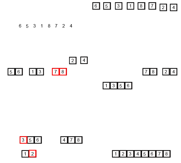
Recursive code like this can often be a little challenging to fully grasp at first so I think it’s worth sharing a pair of visualizations of mergesort that I find helpful. This first is a detailed step by step demonstration of mergesort running on a small list:
 A demonstration of how mergesort operates on small list.
CC BY-SA 3.0
courtesy of Swfung8 on wikipedia.org.
I think that this graphic does a great job of showing how mergesort operates step-by-step: First breaking the list down and then successively building it back up. The second graphic really solidified my understanding of divide and conquer:
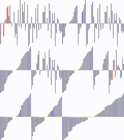
 Another visual representation of mergesort operating on dataset.
This graphic uses a different style of visualization to demonstrate mergesort operating on a larger and more varied dataset. I find it almost hypnotic to watch as the chaotic initial state of the graph is broken up into tiny chunks that increasingly grow larger and more similar as they are trivially compared and combined with their neighbors until the array finally reaches a state of perfect order.
Conclusion
Mergesort is a nice alternative to quicksort in some circumstances and learning about some of the differences and similarities between the two has been a great way to suss out some of the finer points of not only sorting but of computer science algorithms more generally. As always, thanks for reading and please don’t hesitate to reach out to me if you’ve enjoyed what you’ve read or have any other feedback you’d like to share.