Implementing Sorting Algorithms

Lately, I’ve been spending some time trying to better understand the basics of some fundamental sorting algorithms. Sorting algorithms have been a particularly interesting area of study. Sorting an array is a common task and there are a wide variety of well-established sorting algorithms to dig into.

Bubble Sort

I started out looking at bubble sort. Bubble sort is a fairly simple concept—just step through an array comparing each pair of values and swap them if the value at the higher index is less than the value at the lower index. This ends up functioning like this:

CC BY-SA 3.0 courtesy of Swfung8 on wikipedia.org.

As a visual learner, I rigged up a setup for visualizing array changes in javascript and implemented my bubble sort algorithm like this:

function bubbleSort(arr) {
  let length = arr.length;
  //iterate over the entire array n times
  for (let i = 0; i < length; i++) {
    //on each pass, iterate through each element
    for (let j = 0; j < (length - i - 1); j++) {
      //Compare adjacent value pairs
      if (arr[j] > arr[j + 1]) {
        //Swap the numbers
        [arr[j], arr[j + 1]] = [arr[j + 1], arr[j]]
      }
    }
  }
}

In this code, I iterate through the array n times where n is the numer of items in the array. On each loop my code compares each pair of adjacent values and swaps them if the greater value is located in the lower index of the pair. Here is a neat visualization of this exact code executing in a browser-based visualization:

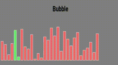Visualization of bubblesorting an unsorted array of integers

Not bad huh? Bubble sort is nice and straight forward but, as you might have reasoned for yourself by now, it is also slow as molasses. As a result of looping through each element of the array n times, bubblesort has an average runtime complexity of O(n²). This abysmal exponential growth means that in the vast majority of scenarios bubble sort is simply not a practical option.

Quick Sort

Quick sort, on the other hand, seems to be on of the most commonly recommended general purpose sorting algorithms with its average runtime complexity of O(n log n). Although in its worst case, quick sort can perform far slower, it is still quite an improvement over bubble sort for the vast majority of workloads. How does quicksort manage such impressive performance gains over bubble sort?

Here is an example demonstrating how quick sort would function on a random array of numbers:

Courtesy of Znupi on wikipedia.org.

What quick sort is doing here can be broken down into three steps:

1. Select a single element, called a pivot, from the array. In this case, the pivot is the rightmost element in the array.
2. Partitioning: reorder the array through sucessive swaps so that all elements with values less than that of the pivot element come before the pivot in the array, while all elements with values greater than that of the pivot come after it.
3. Recursively apply steps one and two to the pair of sub-array of elements with values smaller than the pivot and values larger than the pivot respectively.

Quick sort is classified as a “divide and conquer” algorithm because it efficiently breaks a complex problem down into smaller and smaller problems until they can each be trivially solved a reassembled. This animation can be really helpful in wrapping your head around how that works in practice:

CC BY-SA 3.0 courtesy of RolandH on wikipedia.org.

Quicksort is a bit more complex to implement than bubble sort. I spent a while playing with different approaches to implementing this algorithm and found one in Ruby that was far and away the most simple and elegant:

def quicksort(arr)
  l = arr.size
  return arr if l <= 1
  pivot = arr.delete_at(rand(l))
  left, right = arr.partition {|int| int < pivot }

  return *quicksort(left), pivot, *quicksort(right)
end

That’s it! To understand what this code does let’s take a look at it line by line.

l = arr.size

Here we simply store the size of the array in a variable l.

return arr if l <= 1

This is good hygene to return the array if its size is zero or one because such an array would, by definition, already be sorted but it is also a base case for resolving a recursive call.

pivot = arr.delete_at(rand(l))

This is where things get a bit more fun. In this line, a random element in the array is removed and silmultaneously assigned to the pivot variable. The pivot does not need to be randomly selected but that is what I’ve choosen to do for this implementation.

left, right = arr.partition {|int| int < pivot }

In this line of code, the Ruby method #partition is called on the recently modified array. #Partition is a great Ruby method that can be called on a collection and given a block. The method iterates over each element of the collection, and returns two arrays, the first containing the elements for which the block evaluates to true and the second containing the rest of the elements. In this case, the block splits the two arrays on the basis on whether they are less than the value of the pivot. The resulting arrays are saved as left (less than the pivot) and right (greater than or equal to the pivot)

return *quicksort(left), pivot, *quicksort(right)

In this final line, the method is called recursvely on each of the two partitioned arrays and, when those calls resolve, returns a neat ordered array. The * or splat operators simply indicate that the recursive quicksort calls are otional and thus help us to ensure that our response will be a nice flat array.

Conclusion

There are a number of other sorting algorithms and quicksort is certainly not the be all and end all but I strongly encourage developers to spend a bit of time digging deeper into the logic behind the “sort” functions we so easily take for granted.